ExPDE library
r = Laplace_FE(u) – f;
d = -1.0 * r;
delta = product(r,r);
for(i=1;i<=iteration && delta > eps;++i) {
cout << i << ". ";
g = Laplace_FE(d);
tau = delta / product(d,g);
r = r + tau*g;
u = u + tau * d;
delta_prime = product(r,r);
beta = delta_prime / delta;
delta = delta_prime;
d = beta*d – r;
e = u – u_exakt;
cout << "Iteration: Error: Max:"
<< L_infty(e) << endl;
}
Download
Here you can download version 2.5 of ExPDE.
If you are using this library than please send me an Email.
A first adaptive version of EXPDE will be available at the end of this year.
The development of the library is still in progress.
Therefore suggestions for improving the library are welcome. The library can be compiled with
- GNU g++ compiler (version egcs-2.91.66)
- KAI-compiler
- SGI compiler (MIPSpro Compilers: Version 7.30)
For the parallel version of EXPDE you need MPI.
Here are some versions of MPI, if you want to install MPI:
Efficiency
The efficiency of EXPDE is based on
- semi-unstructured grids and
- expression templates.
Example 1: Parallelization of a cg-solver with multigrid preconditioning for an elasticity equation.
In this example the elasticity equation with Neumann boundary conditions is discretized with linear elements on a semi-unstructured grid. The resulting equation system is solved by cg with a multigrid preconditioner. The following table shows the computational time for one cg-iteration on different meshes and for different number of processors on ASCI Blue-Pacific:
| Number of processors | Number of grid points | Number of unknowns | Time for one cg-iteration |
|---|---|---|---|
| 600 | 121.227.509 | 363.682.527 | 110 sec |
| 131 | 15.356.509 | 46.069.527 | 84 sec |
| 88 | 1.973.996 | 5.921.988 | 18 sec |
| 24 | 1.973.996 | 5.921.988 | 81 sec |
Low computational time by expression templates:
For decreasing the computational time, it is important to avoid the “cache problem” of the computer. To this end, we used a suitable data structure and expression templates. By using expression templates, it is possible to reduce the number of iterations over the discretization grid without a complicated hand optimization of the algorithm. Let us explain this by the following example:
Example 2: One part of the Stokes operator.
For solving the discretized Stokes equation by a multigrid preconditioner one has to evaluate the following system of Laplace operators:
![]()
There are two versions for implementing this system by EXPDE:
Version 1:
f1 = Laplace_FE(u1)  | interior_points;
f2 = Laplace_FE(u2)  | interior_points;
f3 = Laplace_FE(u3)  | interior_points;
Version 2:
f1 = Laplace_FE(u1) &
f2 == Laplace_FE(u2) &
f3 == Laplace_FE(u3) | interior_points;
The following tables depict the computational time of these two versions (the domain ![]() is the domain from here. Furthermore, we used a Ultra 10 SUN workstation).
is the domain from here. Furthermore, we used a Ultra 10 SUN workstation).
| Number of interior grid points |
Computational time in sec of version 1 | Computational time in sec of version 2 |
|---|---|---|
| 232708< | 6.2 | 3.1 |
| 28885 | 0.83 | 0.48 |
| 3530 | 0.16 | 0.09 |
| Increase of the number of interior grid points |
Increase of the computational time of version 1 | Increase of the computational time of version 2 |
|---|---|---|
| 8.05 | 7.48 | 6.4 |
| 8.18 | 5.18 | 5.3 |
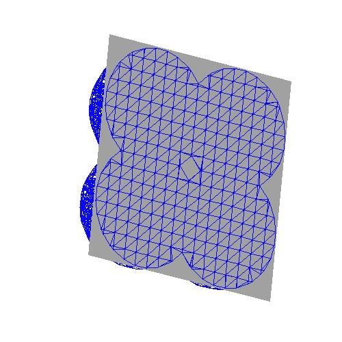
Low storage requirement by semi-unstructured grids:
Semi-unstructured grids consist of a tensor product in the interior of the domain and a minimal unstructured grid near the boundary. On a tensor product grid one can implement discrete FE-differential operators in a very efficient way, without storing the stiffness matrix. Such an efficient implementation is difficult to obtain on an unstructured grid. But, by the construction of the semi-unstructured grid, the unstructured grid near the boundary is a small grid in comparison to the interior grid. Therefore, the computational amount and storage requirement of the unstructured grid can be neglected, if the size of the grid increases.
Example 3: Solving Stokes equation by cg and a multigrid preconditioner
The code of this example can be found in the handbook. The following table depicts the storage requirement with respect to the size of the grid:
| Grid size |
Storage requirement |
||
|---|---|---|---|
| 264600 | 7.2 | 172MB | 7.2 |
| 36673 | 6.8 | 28 MB | 6.1 |
| 5446 | 6.3 | 6.5 MB | 3.4 |
| 846 | /td> | 3.1 MB |
Example 4: Example of a semi-unstructured grid:
The tetrahedrals near the boundary do not have large interior angles. Therefore, the theory and numerical results show optimal approximation properties for semi-unstructured grids.